|
The Shapes Library
Game Physics with Bespoke Code
|
|
The Shapes Library
Game Physics with Bespoke Code
|
This project consists of a collection of basic shapes that can be collided. It's not intended to be a full collision module, but it will give you a sense of some of the math and physics used in collision detection and response. It's implemented as a separate project that compiles to a library file that is linked into the Collision Math Toy and the Pinball Game. Note that unlike the code in the Pool End Game, the collision detection and response code here does not compute exact responses, but instead computes an approximation using faster methods. As a result, tunneling and overlap may occur.
The remainder of this page is divided into five sections. Section 2 lists the controls and their corresponding actions, Section 3 tells you how to build it, Section 4 gives you a list of actions to take in the game to see some of its important features, Section 5 gives a breakdown of the code, and Section 6 addresses the question "what next?".
This project compiles into a library, so there are no keyboard controls here.
This code uses the DirectX12 Toolkit. Make sure that you have followed the instructions in Section 3 of the SAGE Installation Instructions. Note that this project is independent of SAGE. Navigate to the folder 2. Shapes Library in your copy of the sage-physics repository. Run checkenv.bat to verify that you have set the environment variables correctly. Open Shapes.sln with Visual Studio and build the Release and Debug configurations. Alternatively, run Build.bat to build both Release and Debug configurations.
There's no executable file to run here, remember, it just compiles into a library file. If you're interested, the library files are x64\Release\Shapes.lib and x64\Debug\Shapes.lib.
All of the code in this library is in a namespace called Shapes.
ShapeMath.h and ShapeMath.cpp contain some handy helper functions for this project. Since this project is independent of SAGE, some SAGE functions are duplicated here. Of particular interest is FailIf, which will be used inside functions in this project to test a Boolean condition and bail out from the function returning false if the condition is true.
#define FailIf(x) if(x)return false;
This will make our code easier to read when we have multiple failure points within a function.
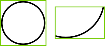
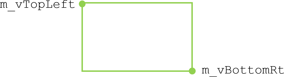
An axially aligned bounding box (AABB for short) is a minimal-size rectanle that bounds a shape and has its edges parallel to the X and Y axes. For example, Fig. 1 shows the AABB for a circle and an arc. AABBs are used in narrow phase collision detection to quickly and efficiently reject things that are too far apart to collide. Our AABBs are implemented by a class Shapes::CAabb2D, which has two private member variables of type Vector2, Shapes::CAabb2D::vTopLeft and Shapes::CAabb2D::vBottomRt which store the coordinates of its top left and bottom right corners as shown in Fig. 2.
AABBs can be built by creating one that encloses a single point using the overloaded assignment operator Shapes::CAabb2D::operator=(), and expanding them to include a new point using Shapes::CAabb2D::operator+=().
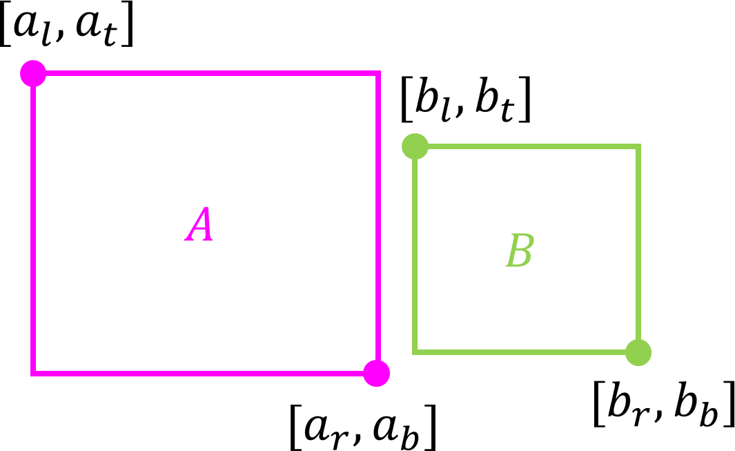
There are two intersection tests involving AABBs which are implemented by overriding Shapes::operator&&. The first one returns true if two AABBs have non-empty intersection: bool operator&&(const CAabb2D&, const CAabb2D&). The best way to think about this is to consider how this function fails, that is, how two AABBs don't intersect. Suppose we have two AABBs \(A\) and \(B\), and that \(A\) has top left corner \([a_l, a_t]\) and bottom right corner \([a_r,a_b]\) and \(B\) has top left corner \([b_l, b_t]\) and bottom right corner \([b_r,b_b]\). One way that \(A\) and \(B\) can be drawn without overlap is for \(A\) to be completely to the left of \(B\), as shown in Fig. 3, in which case \(a_r < b_l\).
Similarly, \(A\) could be completely to the right of \(B\), in which case \(a_l > b_r\); \(A\) could be completely above \(B\), in which case \(a_b > b_t\); or \(A\) could be completely below \(B\), in which case \(a_t < b_b\). These are the only ways that \(A\) can not overlap \(B\). Therefore \(A\) and \(B\) don't intersect iff
\[ (a_r < b_l) \vee (a_l > b_r) \vee (a_b > b_t) \vee (a_t < b_b), \]
That is, using De Morgan's Law, \(A\) and \(B\) do intersect iff
\[ (a_r \geq b_l) \wedge (a_l \leq b_r) \wedge (a_b \leq b_t) \wedge (a_t \geq b_b). \]
This AABB intersection test is therefore extremely fast, using at most four floating point comparisons and three logical operations.
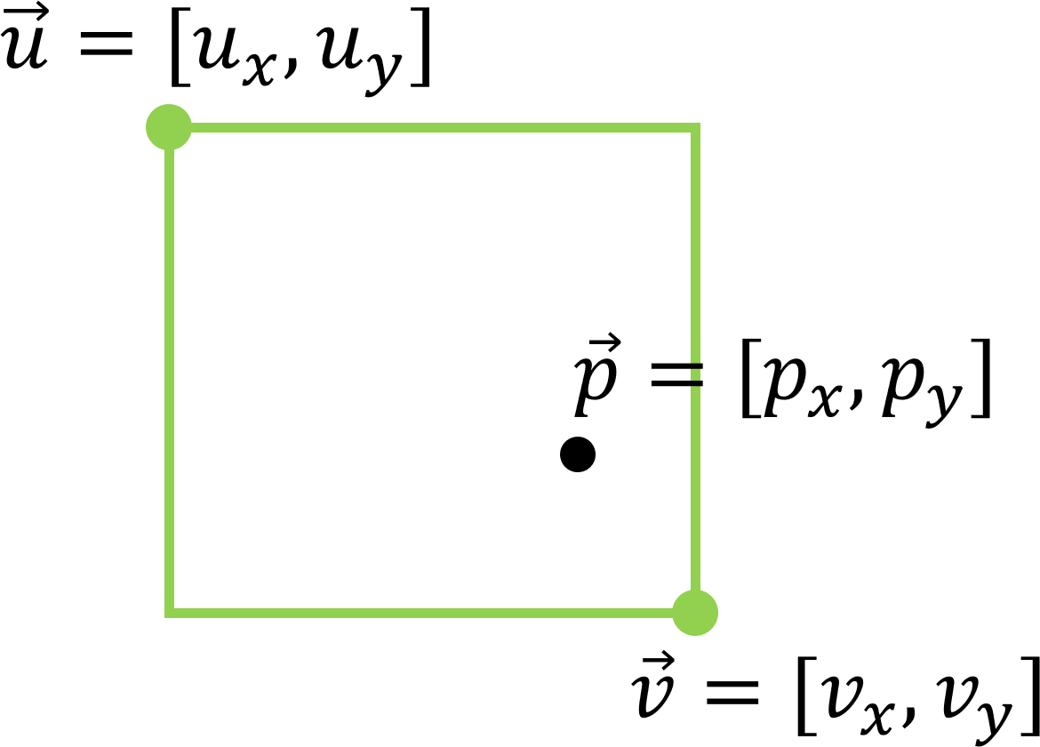
The second AABB intersection test returns true if a point is inside an AABB: bool operator&&(const CAabb2D&, const Vector2&). Suppose the AABB has top left point \([u_x, u_y]\), bottom right point \([v_x, v_y]\), and the point to be tested for intersection with it is \(\vec{p} = [p_x, p_y]\), as shown in Fig. 4.
Then \(\vec{p}\) is inside the bounding box iff
\[ (u_x \leq p_x) \wedge (p_x \leq v_x) \wedge (v_y \leq p_y) \wedge (p_y \leq u_y) \]
The point-in-AABB intersection test is also extremely fast, using at most four floating point comparisons and three logical operations.
The Shapes library has four main shapes: point, line segment, circle, and arc. There is also a line shape for internal use only. Shape types are identified using Shapes::eShape, defined in Shape.h. It also has three motion types, static, kinematic, and dynamic.
Motion types are identified using Shapes::eMotion, also defined in Shape.h.
Shapes::CShapeCommon contains values common to all shapes. Shapes::CShapeDesc is a shape descriptor. Shapes::CShape is the base class for all shapes, from which the static shapes Shapes::CPoint (see Section 5.7), Shapes::CLineSeg (see Section 5.8), Shapes::CCircle (see Section 5.9), and Shapes::CArc (see Section 5.10) are derived.
Shapes::CShape has various protected member variables relating to shapes. Of particular interest are the following.
Shapes::CShape::m_eMotionType, which is initialized to Shapes::eMotion::Static, so that the shapes described in Section 5.7 through Section 5.10 will be static shapes by default. Shapes::CShape::m_eMotionType will be changes to Shapes::eMotion::Kinematic in the constructors of kinematic shapes (see Section 5.11) and to Shapes::eMotion::Dynamic in the constructors of dynamic shapes (see Section 5.12).
Shapes::CShape::m_fElasticity is the "bounciness" of a collision, with 1.0f means a perfectly elastic collision, 0.5f means a collision in which half the velocities are lost in a collision, and values greater than 1.0f mean that a collision imparts extra velocity to the object that it collides with, perhaps by mechanical or electromechanical means, such as a bumper in a pinball machine.
Shapes::CShape::m_bIsSensor. If this is set to true then the shape does not react and does not cause any colliding object to react to a collision with it. This can be used, for example, as a switch to light up lights in a pinball machine.
Shapes::CShape::m_bCanCollide is usually set to true, meaning that the shape can collide with other shapes. Setting it to false will temporarily turn off collisions until it is set to true again. This can be used, for example, for a post that sometimes retracts below the surface in a pinball machine.
Shapes::CShape::m_pUser is a user pointer (that is, a pointer for the use of the programmer) whose aplication will be seen in the Collision Math Toy and the Pinball Machine.
Shapes that can collide with other shapes will have a CollisionDetected function that takes a reference to an instance of the contact descriptor Shapes::CContactDesc that has been initialized with a pointer to the current shape m_pShape and a pointer to the dynamic shape (currently only dynamic circles are implemented) m_pCircle. If the two shapes overlap, CollisionDetected will fill in the other member variables of the contact descriptor as follows and return true. The point of intersection (the coordinates of the point at which the shapes first collided, which is usually between frames) is computed in the 2D vector m_vPOI, the collision normal is computed in m_vNorm, the setback distance (the distance that the dynamic shape must be moved back along the collision normal to its position at the time of impact) is computed in m_fSetback, and the collision speed is computed in m_fSpeed. The main difference between collision detection and response in this project as opposed to the previous one (The 8-ball Pool End Game) is that here the POI will be approximated by the closest point on the shape to the center of the dynamic circle. This is an outrageous fudge, but it looks right in practice and is faster to compute than the alternative.
Shape classes will have various intersection functions that detect overlap with other shapes. Dynamic shapes (the only shapes that can currently react to a collision) They will have a CollisionResponse function that takes as parameter a constant reference to a contact descriptor provided by some call to a CollisionDetected function.
Infinite lines are implemented as class Shapes::CLine, which is for internal use only, that is, for computations internal to the Shapes library. For this reason, Shapes::CLine has no CollisionDetected or CollisionResponse functions, neither does it have any functions to do with updating any member variables, translation, or rotation. It is the only shape that does not have a descriptor and is not derived from Shapes::CShape. Shapes::CLine stores a gradient \(m\), inverse gradient \(1/m\), \(x\)-intercept \(c\), and \(y\)-intercept \(b\). A vertical line has gradient \(m = \infty\) (implemented as float::Inf), \(1/m = 0\), and \(b = \infty\). A horizontal line has gradient \(m = 0\), \(1/m = \infty\), and \(c = \infty\).
The Shapes::CLine constructor takes two parameters, a point \(\vec{p}\) and a floating point gradient \(m\), and initializes its member variables to represent the line of gradient \(m\) through point \(\vec{p}=[p_x, p_y]\). That is, its gradient is \(m\), its inverse gradient \(1/m\), its \(y\)-intercept is \(p_y - p_xm\), and its \(x\)-intercept is \(p_x - p_y/m\).
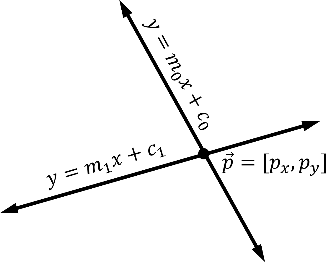
Shapes::CLine::Intersect computes the point of intersection between two lines. If both lines have the same gradient, then there is no point of intersection and the function returns Vector2(Inf, Inf). Otherwise, if neither lines are vertical, and the lines have equations \(y=m_0x + c_0\) and \(y=m_1x+c_1\) as shown in Fig. 5, then the \(x\)-coordinate of the point of intersection of the lines satisfies the equation \(m_0p_x + c_0 = m_1p_x+c_1\), that is, \(p_x = (c_1 - c_0)/(m_0 - m_1)\). The \(y\)-coordinate of the point of intersection is therefore \(p_y = m_0p_x + c_0 = m_0(c_1 - c_0)/(m_0 - m_1) + c_0\).
Otherwise, one of the lines is vertical and the other is not. Suppose the first line is vertical and has equation \(x = c_0\), and that the second line has equation \(y=m_1x+c_1\). Let the point of intersection \(\vec{p}\) have coordinates \([p_x, p_y]\) as shown in Fig. 6.
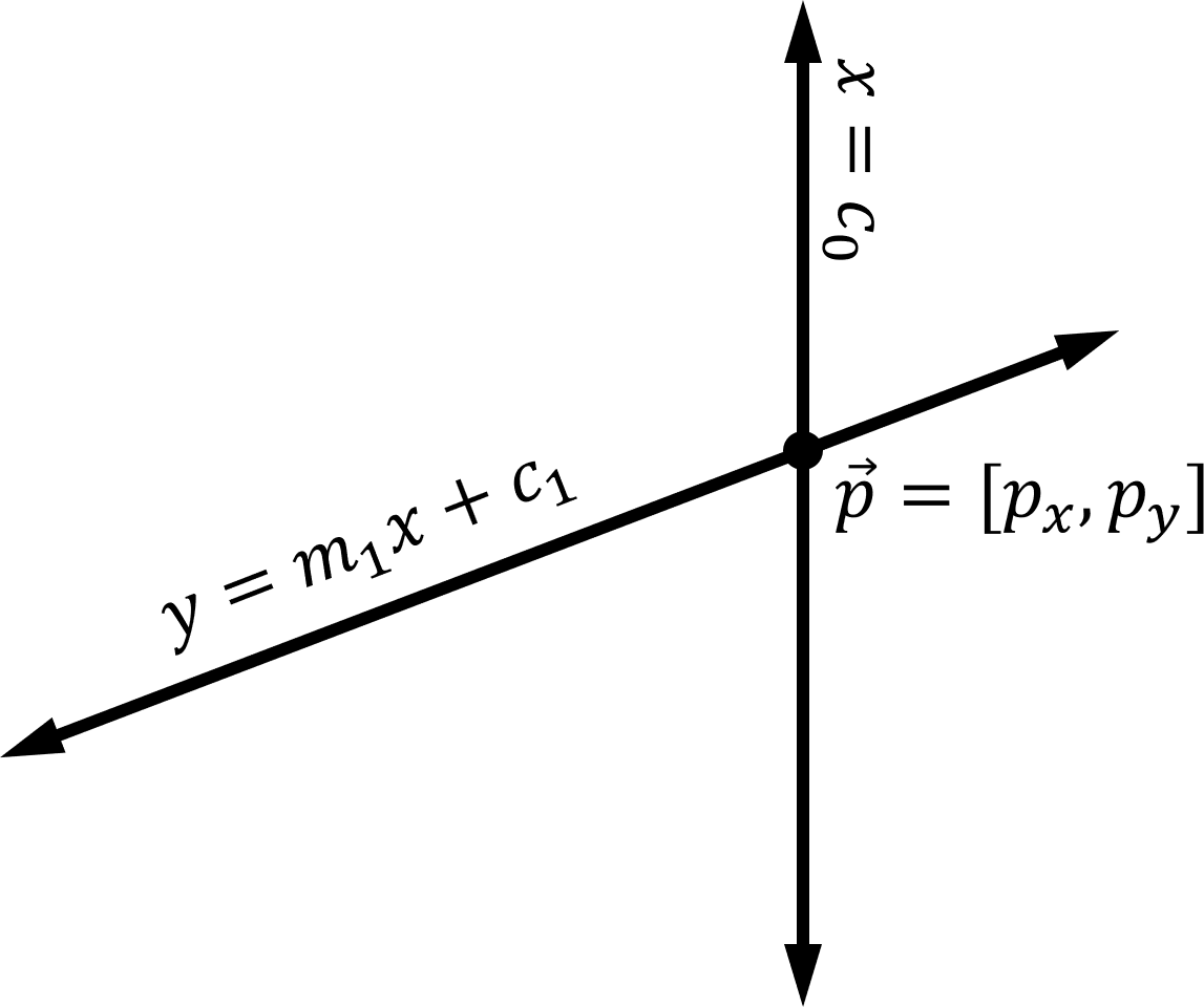
Then \(p_x = c_0\) since \(\vec{p} = [p_x, p_y]\) is on the vertical line \(x = c_0\). Therefore \(p_y = m_1 c_0 + c_1\) since \(\vec{p}\) is on the line \(y=m_1x+c_1\). The case where the second line is vertical and the first line is not vertical is similar.
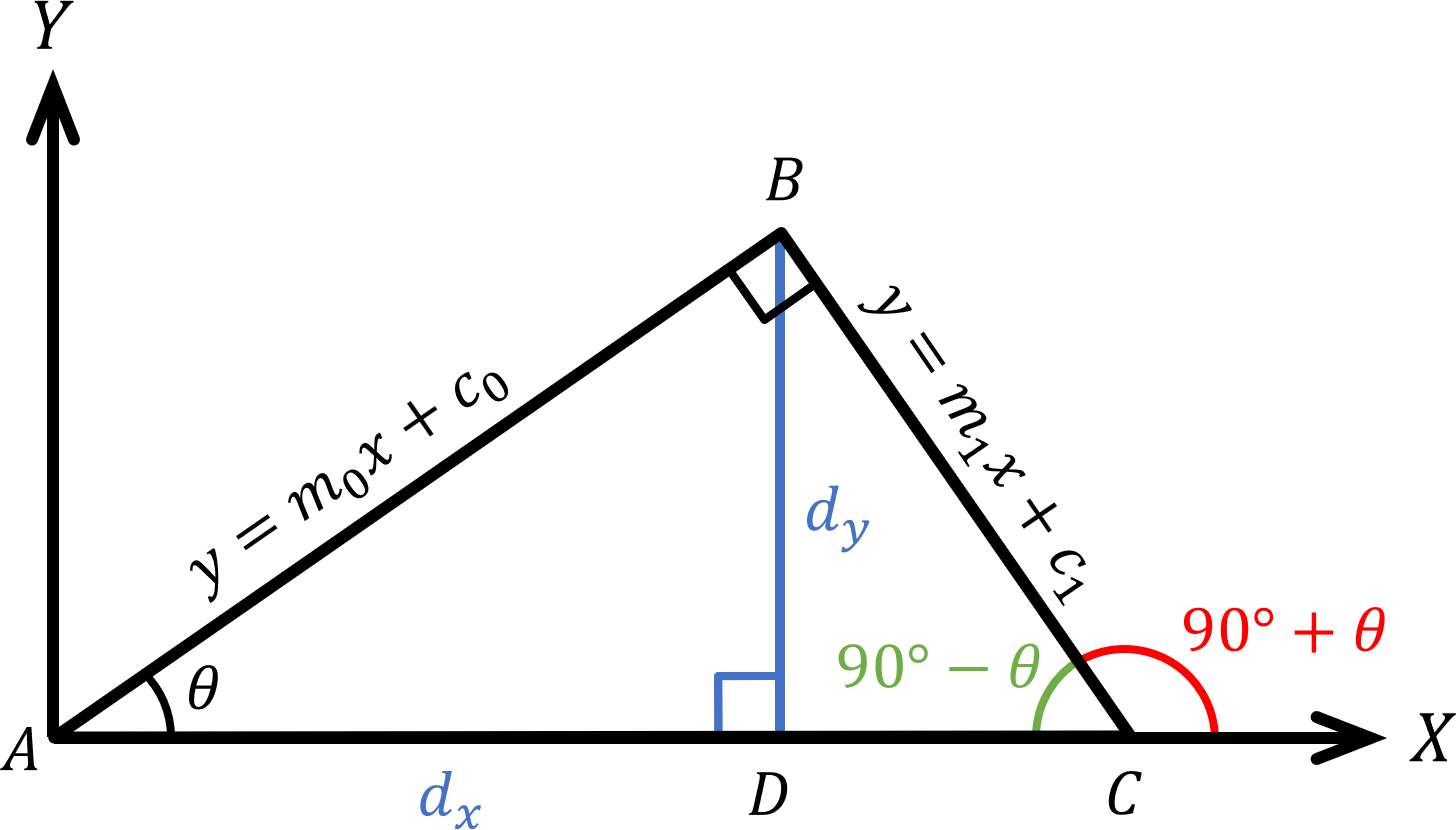
Let \(\triangle ABC\) be the triangle shown in Fig. 7, where \(\overline{AB}\) has equation \(y=m_0x + c_0\), where \(\overline{BC}\) has equation \(y=m_1x + c_1\), and \(\overline{AC}\) lies along the positive \(X\)-axis. Let \(\theta = \angle BAC\). Drop a line perpendicular from \(B\) down to a point \(D\) the \(X\)-axis (shown in blue in Fig. 8). Then, \(\tan \theta = d_y/d_x\) (also shown in blue), that is, rise over run, and so \(m_0 = \tan \theta\). Notice that \(\angle BAC = 90^\circ - \theta\) (shown in green in Fig. 7). Therefore, the angle from the positive \(X\)-axis to \(\overline{BC}\) is \(90^\circ - \theta\) (shown in red in Fig. 7). Since \(\overline{AB}\) has equation \(y=m_0x + c_0\), by an argument similar to the above, \(m_1 = \tan 90^\circ + \theta\). Therefore,
\[ m_1 = \tan (90^\circ + \theta) = \frac{\sin (90^\circ + \theta)}{\cos (90^\circ + \theta)} =- \frac{\cos \theta}{\sin \theta} =\frac{-1}{\tan \theta} =\frac{-1}{m_0}. \]
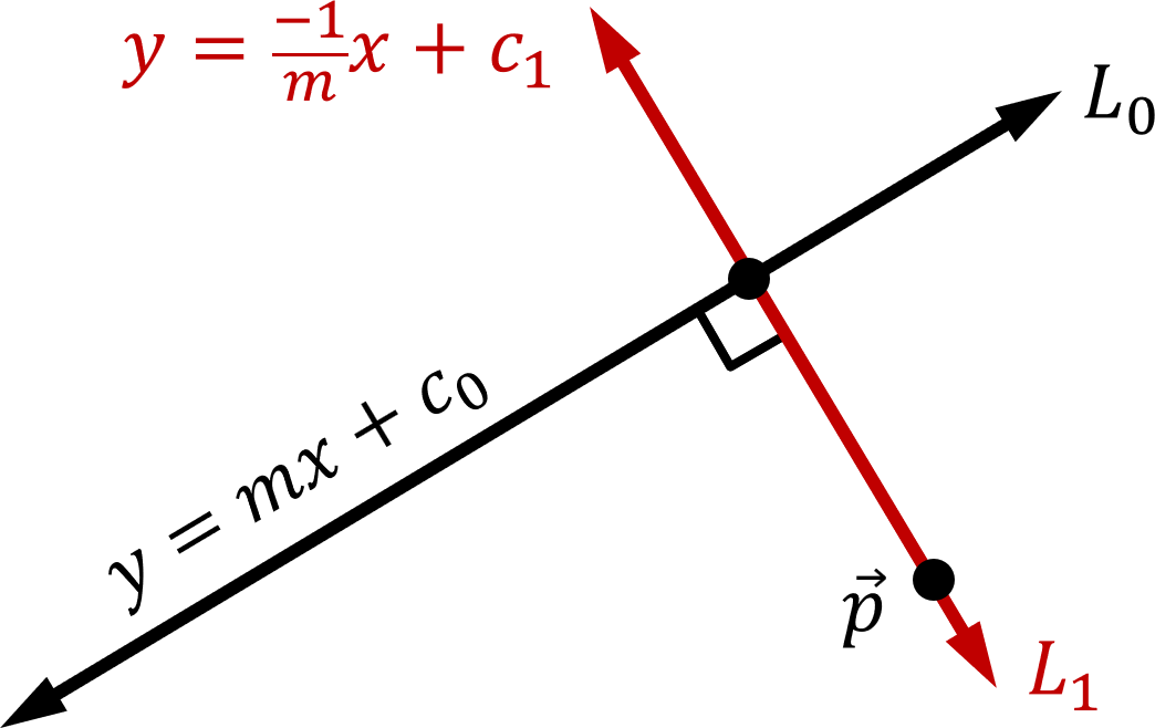
Therefore, as shown in Fig. 8 the closest point on a line \(L_0\) with gradient \(m\) to a point \(\vec{p}\) can be found by computing the point of intersection of the line \(L_0\) with the line \(L_1\) with gradient \(-1/m\) through point \(p\). \(L_1\) is constructed using the Shapes::CLine constructor (see Section 5.6.1) and its point of intersection with \(L_0\) is computed using \(L_0\)'s Shapes::CLine::Intersect function (see Section 5.6.2).
Points are implemented as class Shapes::CPoint, derived from Shapes::CShape. They are instantiated using the descriptor Shapes::CPointDesc. Shapes::CPoint has, in addition to constructors, a collision detection function Shapes::CPoint::CollisionDetected which, as noted in Section 5.5, takes as parameter a reference to an instance of Shapes::CContactDesc initialized with a pointer to a dynamic circle and fills in the POI, collision normal, and setback distance.
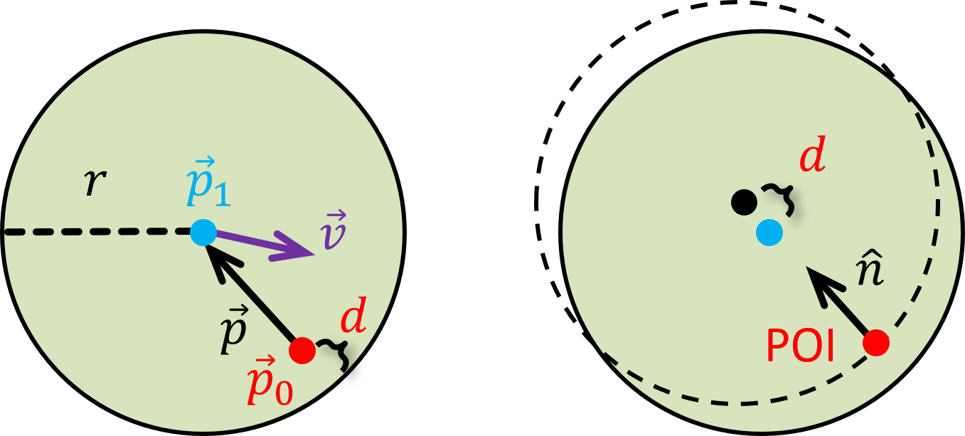
If we assume that the circle and the point are moving relatively slowly, then the point will be only a short distance in from the edge of the circle when the collision is detected, as shown in Fig. 9, left. In that figure the circle (in green) has radius \(r\) and center point \(\vec{p}_1\) (blue) and it is moving at velocity \(\vec{v}\) rightwards and slightly down (purple) towards point \(\vec{p}_0\) (red). Shapes::CPoint::CollisionDetected computes \(\vec{p} = \vec{p}_1 - \vec{p}_0\), the vector from \(\vec{p}_0\) to \(\vec{p}_1\). A collision is detected when \(||\vec{p}|| < r\). The POI is taken to be the coordinates of \(\vec{p}_0\) at the time the collision is detected, the setback distance is taken to be \(r - || \vec{p} ||\), the collision normal is taken to be \(\hat{p}\), and the collision speed is \(||\vec{p}_0 ||\). These are mostly not the correct values but, as we will see later in the Collision Math Toy and the Pinball Game, are usually close enough.
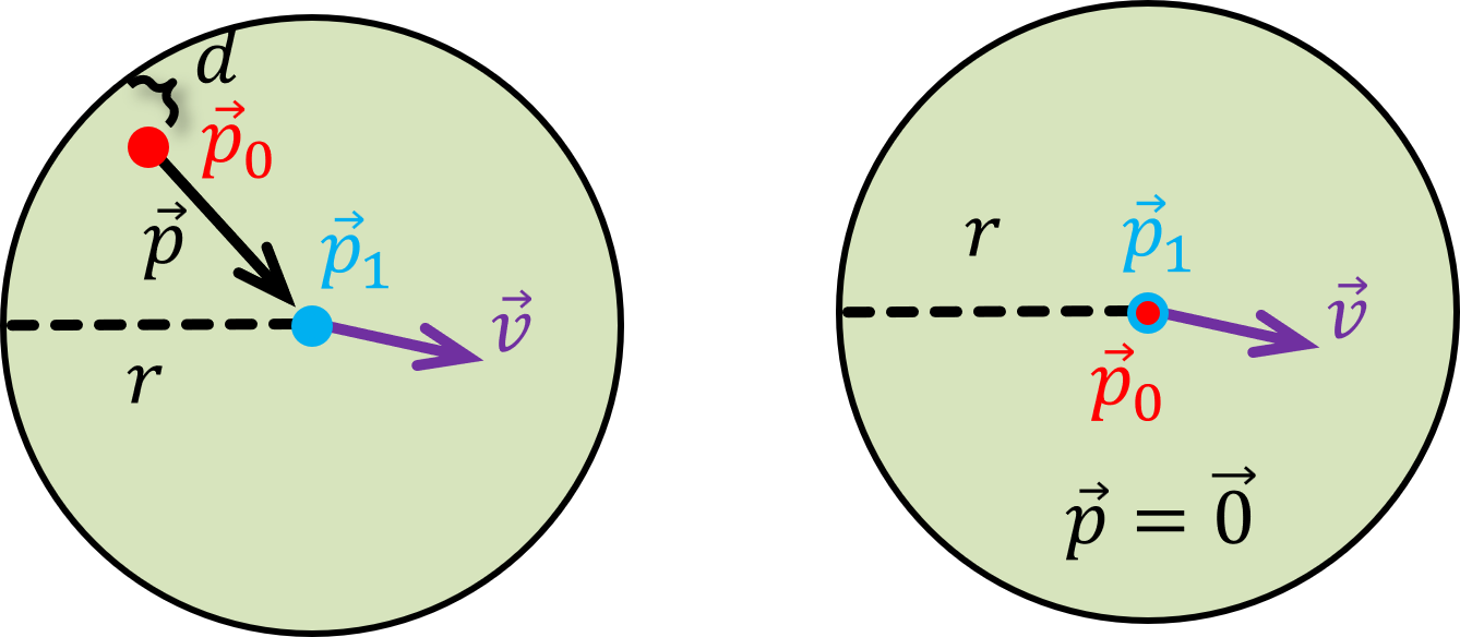
However, if our assumption that the circle and the point are moving relatively slowly is incorrect, then there are a number of things that can go wrong. For example, the circle could completely travel through the point without a collision being detected (tunneling), or it could travel almost competely through the point as shown in Fig. 10, left (in which case the circle will be reflected in the wrong direction), or \(\vec{p}_0\) could be very close to or equal to \(\vec{p}_1\) as shown in Fig. 10, right (in which case we may get a divide-by-zero).
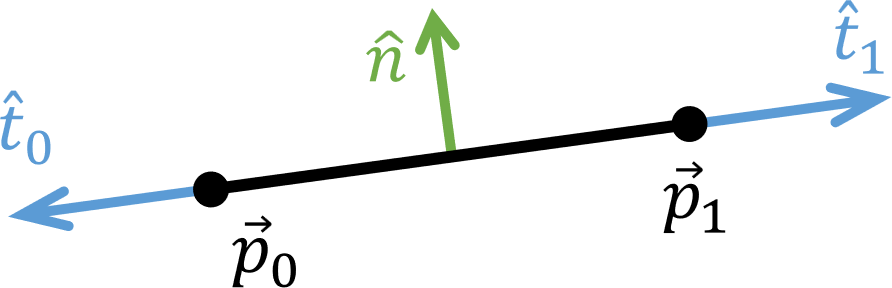
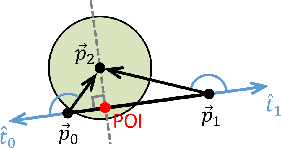
Line segments are implemented as class Shapes::CLineSeg, derived from Shapes::CShape and Shapes::CLine (see Section 5.6). They are instantiated using the descriptor Shapes::CLineSegDesc. Shapes::CLineSeg stores, in addition to inherited values, the coordinates of the end points \(\vec{p}_0\) and \(\vec{p}_1\), the corresponding tangent vectors \(\hat{t}_0\) and \(\hat{t}_1\), and the counterclockwise normal \(\hat{n}\) from \(\vec{p}_0\), noting that we will always enforce the condition that \(\vec{p}_0\) will always be to the left of, or at the same \(X\)-coordinate as \(\vec{p}_1\) as shown in Fig. 11. Note that \(\hat{t}_0 = - \hat{t}_1\) and \(\hat{t}_0 \cdot \hat{n} = \hat{t}_1 \cdot \hat{n} = 0\).
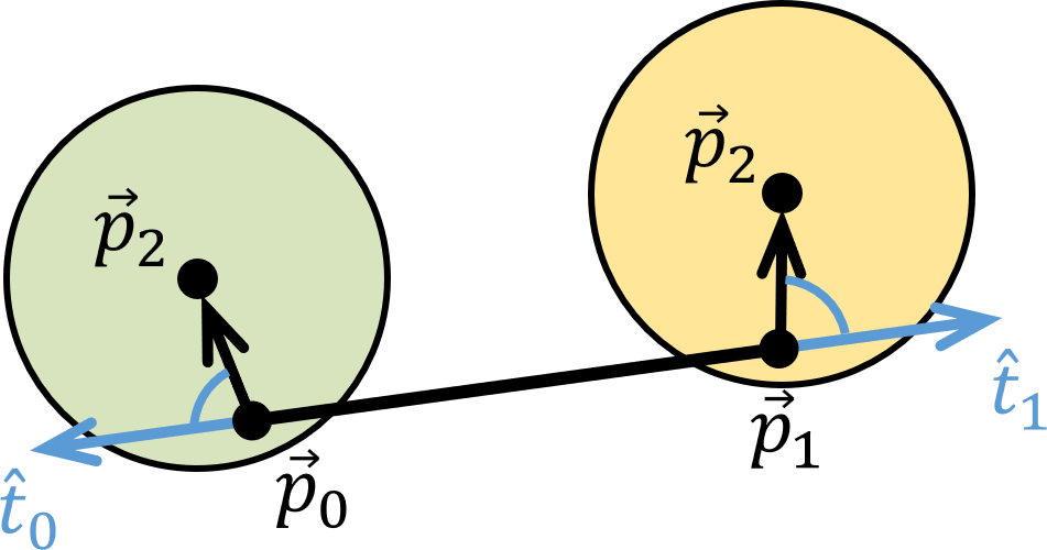
Shapes::CLineSeg has, in addition to constructors and reader functions, a collision detection function Shapes::CLineSeg::CollisionDetected which, as noted in Section 5.5, takes as parameter a reference to an instance of Shapes::CContactDesc initialized with a pointer to a dynamic circle and fills in the POI, collision normal, and setback distance. Shapes::CLineSeg::CollisionDetected rejects collisions with dynamic circles that approach from the ends of the line segment, that is, if the circle center is \(\vec{p}_2\), either \((\vec{p}_2 - \vec{p}_0)\cdot \hat{t}_0 < 0\) or \((\vec{p}_2 - \vec{p}_1)\cdot \hat{t}_1 < 0\), as shown in Fig.12.
Otherwise \((\vec{p}_2 - \vec{p}_0)\cdot \hat{t}_0 \geq 0\) and \((\vec{p}_2 - \vec{p}_1)\cdot \hat{t}_1 \geq 0\), in which case we take the POI to be the closest point on the line segment to \(p_2\), as shown in Fig.13, using a call to Shapes::CLine::ClosestPt. We then foist the rest of the work to Shapes::CPoint, as follows.
return CPoint(CPointDesc(ClosestPt(p2))).CollisionDetected(c);
where c is the contact descriptor for this collision.
Circles are implemented as class Shapes::CCircle, derived from Shapes::CShape. They are instantiated using the descriptor Shapes::CCircleDesc. Shapes::CCircle stores, in addition to inherited values, its radius m_fRadius and the square of the radius m_fRadiusSq, the purpose of which will become clear in Section 5.9.1. It also has some useful public member functions, including Shapes::CCircle::PtInCircle test, a Shapes::CCircle::ClosestPt function Shapes::CCircle also has a collision detection function Shapes::CCircle::CollisionDetected which, as noted in Section 5.5, takes as parameter a reference to an instance of Shapes::CContactDesc initialized with a pointer to a dynamic circle and fills in the POI, collision normal, and setback distance.
Shapes::CCircle::PtInCircle checks whether a point \(\vec{p}_1=[x_1, y_1]\) is inside the circle by checking whether the distance from \(\vec{p}_1\) to the center of the circle \(\vec{p}_0=[x_0,y_0]\) is less than the radius \(r\). That is, whether
\[ \sqrt{(x_0 - x_1)^2 + (y_0 - y_1)^2} < r. \]
To save doing the potentially costly square-root, we test instead whether
\[ (x_0 - x_1)^2 + (y_0 - y_1)^2 < r^2, \]
noting that the radius squared is computed and stored in m_fRadiusSq in the constructor, and that DirectX::SimpleMath::Vector2 has a function LengthSquared to compute the square of its length.
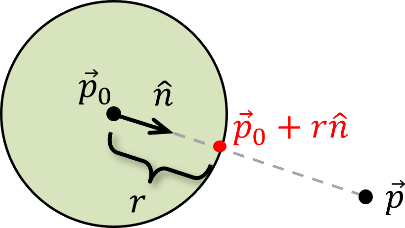
Shapes::CCircle::ClosestPt finds the closest point on the perimeter to the point \(\vec{p}\) as follows. Suppose the center of the circle is \(\vec{p}_0\). Compute \(\vec{n} = \vec{p}_0 - \vec{p}\), the vector from \(\vec{p}_0\) to \(\vec{p}\), and normalize it to get \(\hat{n}\). Then the point on the perimeter closest to \(\vec{p}\) is \(\vec{p}_0 + r\hat{n}\), as shown in Fig. 14.
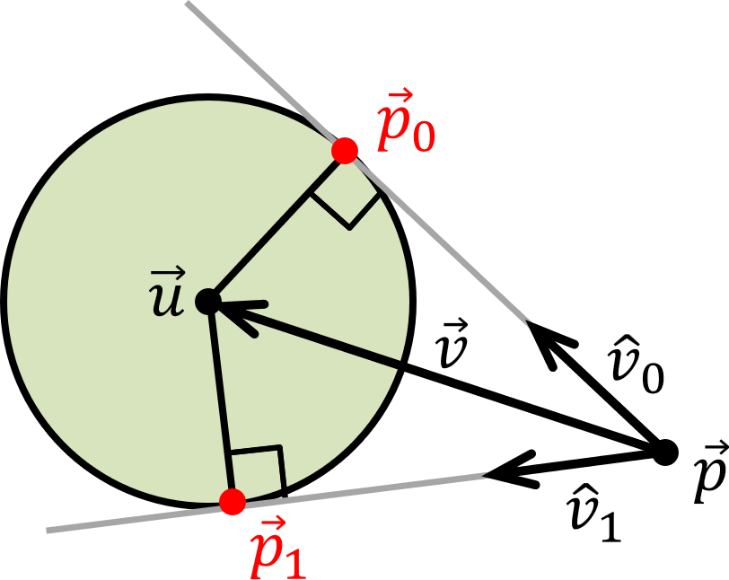
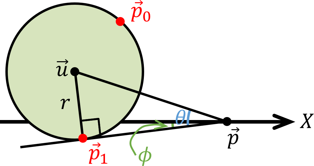
Shapes::CCircle::Tangents(const Vector2&, Vector2&, Vector2&) finds the intersection points \(\vec{p}_0, \vec{p}_1\) of the tangents to a circle of radius \(r\) and center \(\vec{u}\) through an exterior point \(\vec{p}\). Let \(\vec{v} = \vec{u} - \vec{p}\) be the vector from \(\vec{p}\) to \(\vec{u}\). Let \(\hat{v_0}\) be the unit vector that points along the tangent from \(\vec{p}\) to \(\vec{p}_0\) and let \(\hat{v_1}\) be the unit vector that points along the tangent from \(\vec{p}\) to \(\vec{p}_1\). This is depicted in Fig.15.
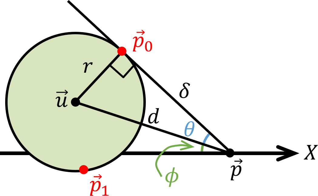
Consider the first of these points \(\vec{p}_0\). Consider the triangle with vertices \(\vec{p}\), \(\vec{p}_0\), and \(\vec{u}\) as shown in Fig. 16. The length of the hypotenuse \(d\) is equal to the length of the vector \(\vec{v}\) from \(\vec{p}\) to \(\vec{u}\), that is, \(d = ||\vec{u} - \vec{p}||\). Let \(\delta\) be the length of the tangent through \(\vec{p}\) and \(\vec{p}_0\). Since the triangle is a right triangle, we know by the Pythagorean Theorem that \(\delta^2 + r^2 = d^2\), that is, \(\delta = d^2 - r^2\). Also since the triangle is a right triangle, the tan of the angle \(\theta\) shown in blue in Fig.16 is \(r/\delta\), and therefore \(\theta = \arctan (r/\delta)\). The angle between the positive \(X\)-axis and the line between \(\vec{p}\) and \(\vec{u}\) is \(\phi = \arctan(v_y/v_x)\), shown in green in Fig.16. Therefore, the angle between the positive \(X\)-axis and the tangent is \(\theta + \phi\), and \(\hat{v_0} = [\cos(\theta + \phi), \sin(\theta + \phi)]\). Then to get from point \(\vec{p}\) to point \(\vec{p}_0\) we need to go a distance of \(\delta\) in the direction of \(\hat{v}_0\), that is, \(\vec{p}_0 = \vec{p} + \delta \hat{v}_0\).
The computation of the second of these points \(\vec{p}_1\) is similar to the above, except that \(\hat{v_1} = [\cos(\theta - \phi), \sin(\theta - \phi)]\), noting that in Fig. 17, \(\theta\) is the positive angle between \(\vec{v}\) and \(\hat{v}_1\) and \(\phi\) is the positive angle between the \(X\)-axis and \(\hat{v}_1\).
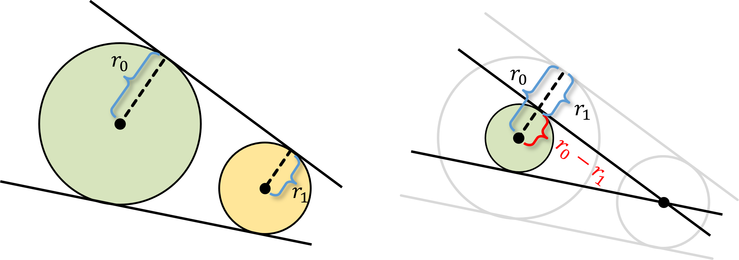
Shapes::CCircle::Tangents(const CCircle*, CLineSegDesc&, CLineSegDesc&) computes the line segments for the tangents to two circles of radius \(r_0\) and \(r_1\), where \(r_1 < r_0\), as shown in Fig. 18, left. J. Casey, A sequel to the First Six Books of the Elements of Euclid, pp. 31-32, 1888 notes that you can shrink both circles by the same amount and maintain exactly the same tangents. As observed in Fig. 18, right, you can shrink the smaller (yellow) circle down to a single point while shrinking the larger (green) circle down to radius \(r_0 - r_1\). This reduces the problem to that of finding the intersection points of the tangents of a circle through an external point, which we can solve using the method of Section 5.9.3.
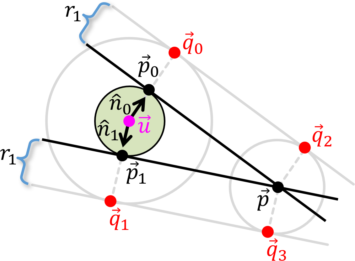
Suppose the points of intersection on the reduced large circle are \(\vec{p}_0, \vec{p}_1\) and its center is at position \(\vec{u}\), as shown in Fig. 19. Compute \(\vec{n}_0 = \vec{p}_0 - \vec{u}\) and \(\vec{n}_1 = \vec{p}_1 - \vec{u}\) and normalize them to get \(\hat{n}_0\) and \(\hat{n}_1\). Then the points of intersection of the common tangents of the two circles are \(\vec{q}_0 = \vec{p}_0 + r_1 \hat{n}_0\) \(\vec{q}_1 = \vec{p}_1 + r_1 \hat{n}_1\) on the large circle and \(\vec{q}_2 = \vec{p} + r_1 \hat{n}_0\) \(\vec{q}_3 = \vec{p} + r_1 \hat{n}_1\), again as shown in Fig. 19.
As we did with line segments (see Section 5.8), Shapes::CCircle::CollisionDetected foists off the work of filling in the collision descriptor c to an instance of Shapes::CPoint for the closest point on the dynamic circle to the center of this circle, as follows.
return CPoint(ClosestPt(c.m_pCircle->GetPos())).CollisionDetected(c);
As before, this is not the correct POI but we will see in later projects that it is close enough.
Arcs are implemented as class Shapes::CArc, derived from Shapes::CCircle (see Section 5.9). They are instantiated using the descriptor Shapes::CArcDesc.
Arcs are defined by a pair of angles, for example, the angles \(\alpha_0\) and \(\alpha_1\) shown in Fig. 20. Note that at all times we will ensure that the stored values of these angles in Shapes::CArcDesc and Shapes::CArc always have the property that \(0 \leq \alpha_0, \alpha_1 < 2\pi\). As shown in Fig. 20, we always store the coordinates of the end points of the arc \(\vec{p}_0\) and \(\vec{p}_1\), respectively, and the tangents to the arc at those points \(\vec{t}_0\) and \(\vec{t}_1\), respectively. To facilitate consistency is maintained when we rotate an arc in Shapes::CKinematicArc, the angles, points, and tangents will be stored in private member variables that are updated together automatically using Set functions. This is not formally allowed in our definition of a Descriptor, but as Ralph Waldo Emerson once said, "Consistency is the bugbear of tiny minds."
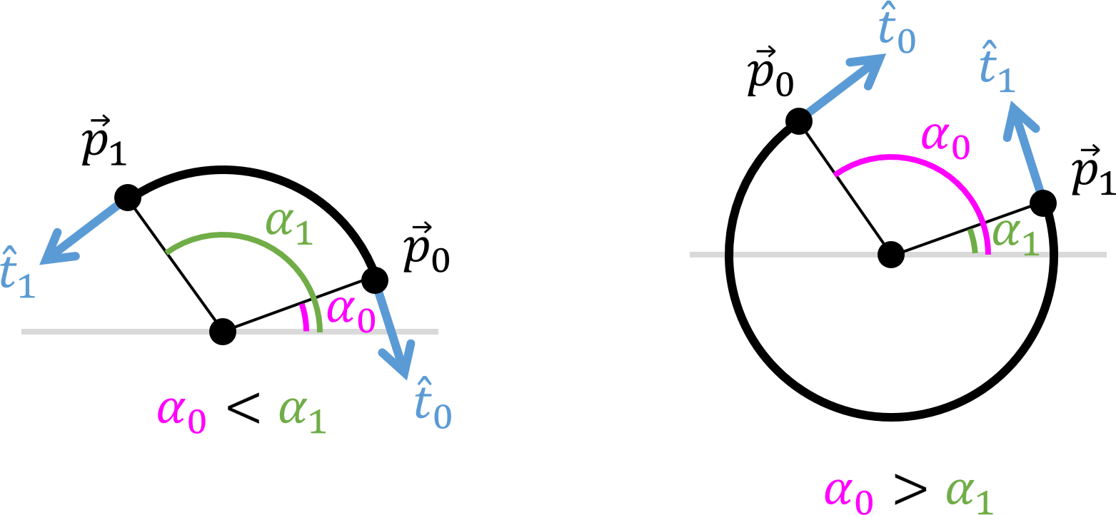
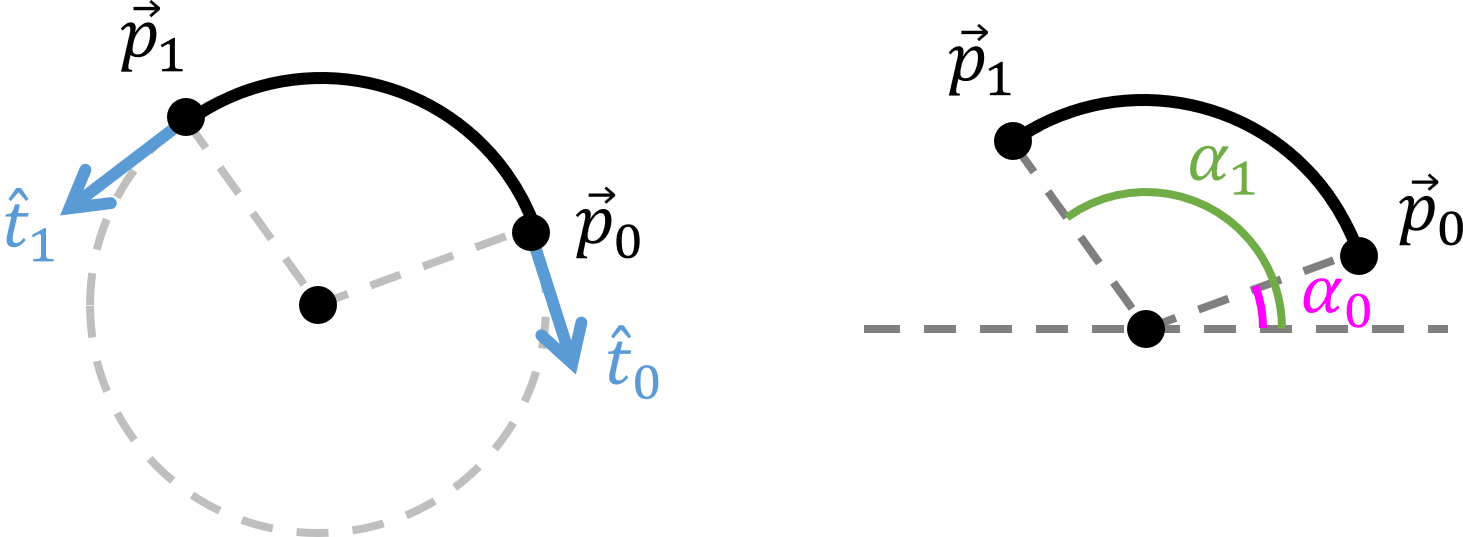
Note that our definition of arc so far is ambiguous: the arc could be either the smaller or larger portion of a circle. Our code will adopt the convention that the arc is that part of the perimeter of a circle that goes counterclockwise from \(\vec{p}_0\) to \(\vec{p}_1\). Therefore, flipping the arc from one portion of a circle to its complement means just swapping the angles and swapping and reversing the direction of the normals. For example, in Fig. 21 (left) we have the case that \(\alpha_0 < \alpha_1\), while in Fig. 21 (right) \(\alpha_0 > \alpha_1\). For convenience, we will call the former an acute arc and the latter an obtuse arc.
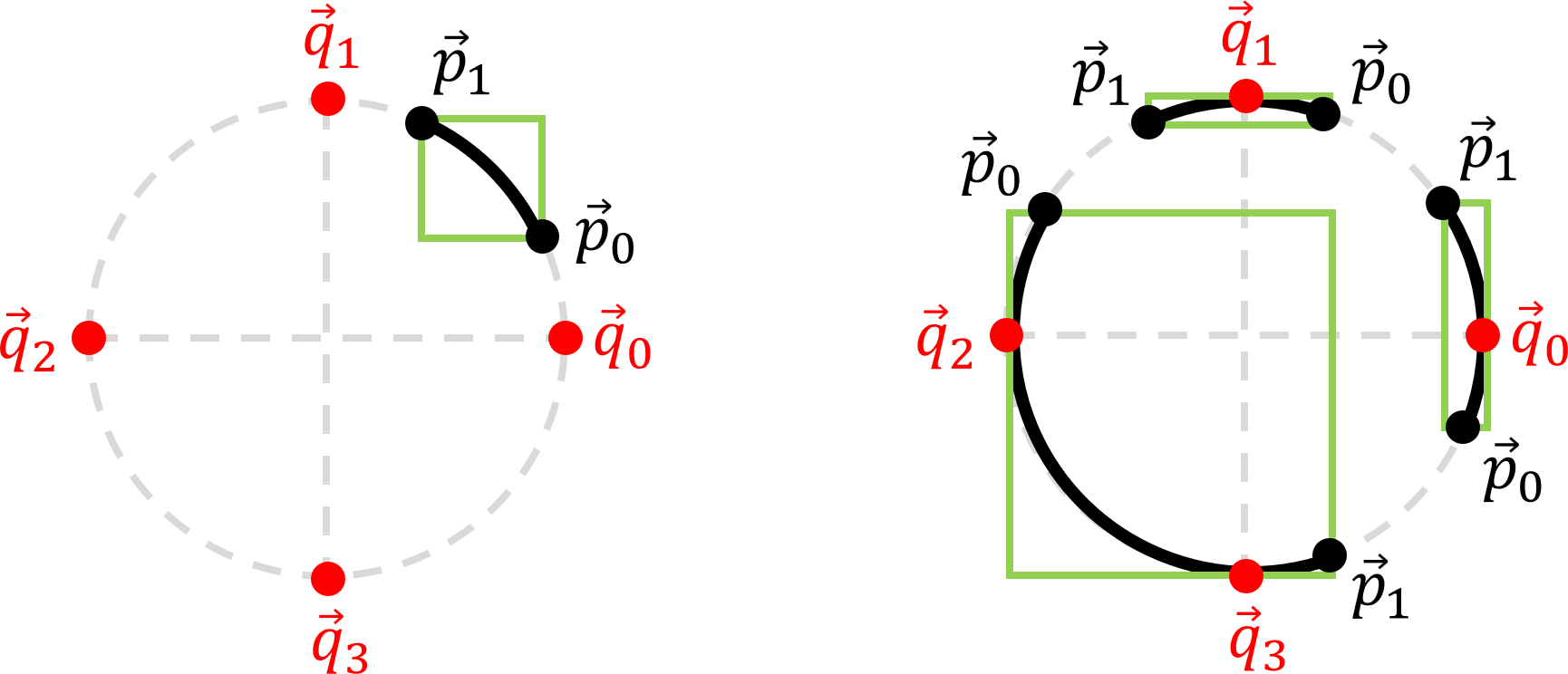
Function Shapes::CArc::Update computes the arc's end points, tangents, and AABB from its center point and angles. The trickiest of these is the AABB. Consider the arc shown in Fig. 22, left. Since none of what we will call quadrant points, the four points on the extreme left, right, top, and bottom of the circle containing the arc (shown in red), then the AABB of the arc (shown in green) is just the smallest AABB that contains the end points of the arc \(\vec{p}_0\) and \(\vec{p}_1\). Fig. 22, right, shows three arcs that do overlap one or more of the quadrant points. Clearly, their AABBs must be the smallest AABB that includes their respective end points and whichever quadrant points lie on the arc.
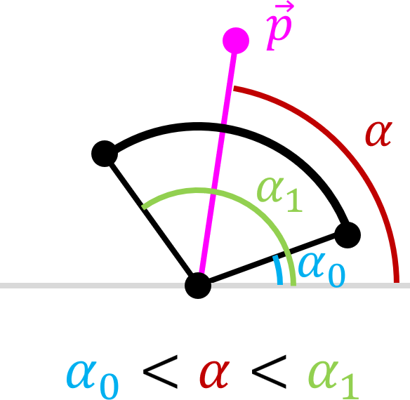
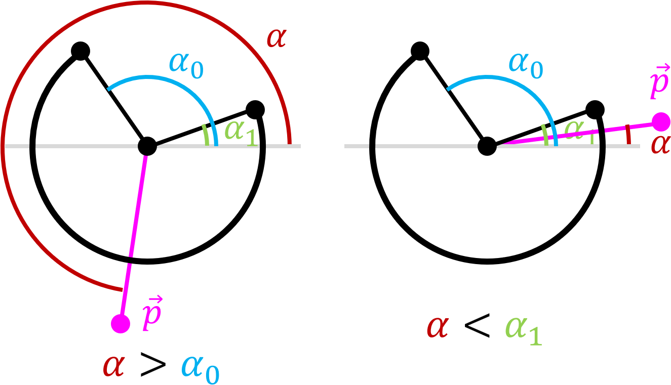
Function Shapes::CArc::PtInSector determines whether the coordinates of a point \(\vec{p}\) lie within the sector of the arc, which depends on whether the arc is acute or obtuse (refer back to Section 5.10.1 for definitions). It begins by finding the orientation \(\alpha\) of the vector from the center of the arc to \(\vec{p}\). Suppose the arc angles are \(\alpha_0\) and \(\alpha_1\). If \(\alpha_0 < \alpha_1\), then the arc is acute and \(\vec{p}\) is within the sector of the arc iff \(\alpha_0 \leq \alpha \leq \alpha_1\) (see Fig. 24).
Otherwise, the arc is obtuse and \(\vec{p}\) is within the sector of the arc iff \(\alpha_0 \leq \alpha \) or \(\alpha \leq \alpha_1\) (see Fig. 25).
Shapes::CArc::CollisionDetected begins by rejecting the collision if the dynamic circle comes from outside the arc sector or is inside the arc circle and is approaching in the direction opposite a tangent to the arc. This is to avoid overlap with the end of the arc as much as possible. Otherwise the POI is taken to be the point on the arc closest to the center of the dynamic circle, and the work of filling in the collision descriptor c is once again foisted off to an instance of Shapes::CPoint for the POI.
return CPoint(ClosestPt(c.m_pCircle->GetPos())).CollisionDetected(c);
As before, this is not the correct POI but we will see in later projects that it is close enough.
The Shapes Library includes the following kinematic shapes Shapes::CKinematicPoint, Shapes::CKinematicLineSeg, Shapes::CKinematicCircle, and Shapes::CKinematicArc. Each kinematic shape is derived from the corresponding static shape described in Section 5.10 and inherits Shapes::CShape::m_eMotionType which is set to Shapes::eMotion::Kinematic in the constructor. Each kinematic shape has additional private member variables in which the relevant constructor stores its initial position and/or orientation at time of instantiation.
Every kinematic shape has a Reset function that resets its current position and orientation to the initial ones and a Rotate function that takes the coordinates of the center of rotation and an angle to be added to the initial orientation to get the current orientation. Shapes::CKinematicPoint::Rotate and Shapes::CKinematicCircle::Rotate both use a single call to Shapes::RotatePt to rotate their positions. Shapes::CKinematicArc::Rotate also changes the arc angle and calls Shapes::CArc::Update as the last thing. Shapes::CKinematicLineSeg::Rotate rotates its end points (not its position), swaps the points if they are out of order, recomputes the position and lastly calls Shapes::CLineSeg::Update.
The only dynamic shapes implemented so far in the Shapes Library is Shapes::CDynamicCircle, which is derived from Shapes::CCircle and has its own descriptor Shapes::CDynamicCircleDesc. It has private member variables Shapes::CDynamicCircle::m_vVel for its velocity and Shapes::CDynamicCircle::m_fMass for its mass. The most interesting part of Shapes::CDynamicCircle is its collision response functions. Public member function Shapes::CDynamicCircle::CollisionResponse takes as parameter a const reference to a contact descriptor that describes the collision. This is passed to private member functions Shapes::CDynamicCircle::CollisionResponseStatic, Shapes::CDynamicCircle::CollisionResponseKinematic, or Shapes::CDynamicCircle::CollisionResponseDynamic, depending on whether the shape that this dynamic circle is colliding with is, respectively, static, kinematic, or dynamic.
Shapes::CDynamicCircle::CollisionResponseStatic computes a dynamic circle's response to collision with a static shape. The dynamic circle is moved along the contact normal by the setback distance. If the dynamic circle is moving towards to POI, then its velocity is flipped and multiplied by the product of the dynamic circle and the static shape's elasticity.
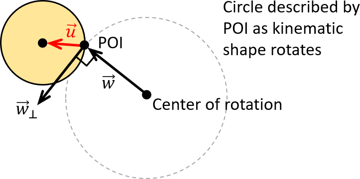
Shapes::CDynamicCircle::CollisionResponseKinematic computes a dynamic circle's response to collision with a kinematic shape. It first calls Shapes::CDynamicCircle::CollisionResponseStatic to modify the dynamic circle's position and velocity as if the kinematic shape were static. It then gives an extra kick to the dynamic circle's velocity from the kinematic shape's rotation delivered through the POI (see Fig. 26). Let \(\vec{w}\) be the vector from the kinematic shape's center of rotation to the POI and let \(\vec{w}_\perp\) be the counterclockwise perpendicular to \(\vec{w}\), computed using Shapes::perp. Suppose the kinematic shape has rotation speed \(a\) rotations per second. Then the velocity of the POI at time of impact is \(2 \pi a \vec{w}_\perp\) (remembering that the length of \(\vec{w}_\perp\) is the radius of rotation). Therefore, the velocity of the POI relative to the dynamic circle is \(\vec{v}_1 = 2 \pi a \vec{w}_\perp - \vec{v}\), where \(\vec{v}\) is the velocity of the dynamic circle. Let \(\vec{v}_2\) be the component of \(\vec{v}_1\) parallel to \(\vec{u}\) the vector from the POI to the center of the dynamic circle shown in red in Fig. 26. Then the product of \(\vec{v}_2\) times the elasticities of the shapes is added to the velocity \(\vec{v}\) of the dynamic circle.
Shapes::CDynamicCircle::CollisionResponseDynamic computes a dynamic circle's response to collision with a dynamic shape. The code here is similar to the response code in NarrowPhase in the Pool End Game, with the major change being the fact that the balls may have different masses, and so we use the formula from Section 2 of Newtons's Cradle and Friends instead of Section 1.
Shapes::CCompoundShape consists of an std::vector of shapes and some public functions that can be used to rotate the whole shape as if it were kinematic. This is mainly for convenience.
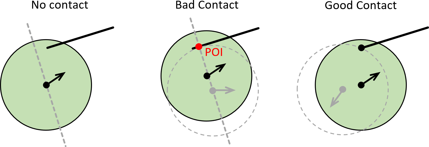
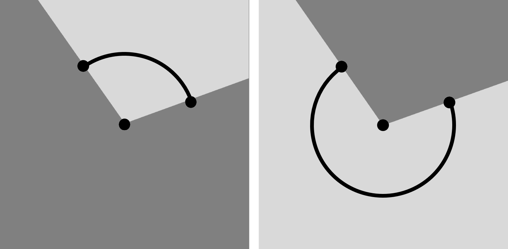
You will notice from the above that collisions that involve a dynamic circle colliding with the ends of a line segment (Section 5.8) or arc (Section 5.10.4) are rejected. For example, dynamic circle collide with line segment is done by finding the closest point to the center of the circle on the line through the line segment and rejecting it if it is not on the line segment, as shown in Fig.27, left. Even worse, the dynamic circle may move from there so that the POI is actually on the line segment, shown in red in Fig.27, middle. The collision response for the dynamic circle will place it in the grey dotted circle with velocity away from the line segment. This usually results in a large jump in position so that the dynamic circle skims off the edge of the line segment. What we really want is for the dynamic circle to bounce off the end of the line segment, as shown in Fig.27, right. For this to happen, the programmer needs to actually place an instance of Shapes::CPoint there and make sure that collision detection of dynamic shapes and points is done before dynamic shapes and line segments or arcs. We will call a line segment or arc without instances of Shapes::CPoint to protects its ends a naked shape.
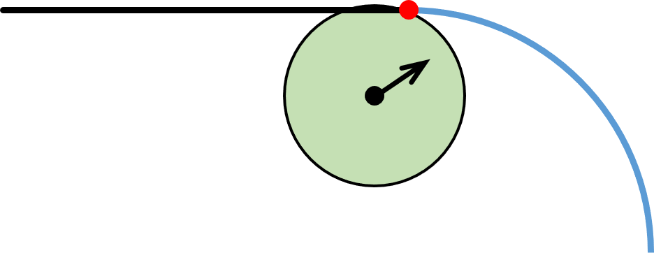
However, there are places in which a guard point is unnecessary and may actually give incorrect behavior. This includes arcs and line segments that are share an end point and are tangent to other arcs or line segments. For example, in Fig. 28, if the red dot is an instance of Shapes::CPoint then the green circle may bounce off it and recoil leftwards and down instead of rightwards and down.
Next, take a look at the Collision Math Toy.