1. Introduction

Fig. 1: Bodies made up from springs and sticks.

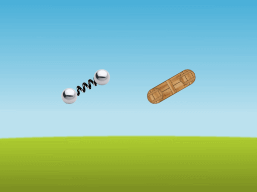
The Ball and Spring Toy applies Verlet integration and Gauss-Seidel Relaxation to bodies made up of balls connected by springs and sticks. The bodies fall under gravity and you can apply a random impulse to them to see how they react The types of bodies available are chains of length 2, 3, and 4; wheels of size 4, 5, and 6; and a ragdoll robot (see Fig. 1). For each body type except the ragdoll robot you are given two bodies, one with springs and one with sticks. The ragdoll robot has some primitive AI that attempts to make it stand up and move to the center of the window.

The remainder of this page is divided into five sections. Section 2 lists the controls and their corresponding actions, Section 3 tells you how to build it, Section 4 gives you a list of actions to take in the game to see some of its important features, Section 5 gives a breakdown of the code, Section 6 contains some programming problems, and Section 7 addresses the question "what next?".

2. Controls

Key	Action
F1	Help (this document)
Backspace	Restart with the current body type
Enter	Advance to the next body type
Space	Apply a random impulse
P	Save screenshot to a file
Esc	Quit game and close the window

3. Building the Game

This code uses SAGE. Make sure that you have followed the SAGE Installation Instructions. Navigate to the folder 5. Ball and Spring Toy in your copy of the sage-physics repository. Run checkenv.bat to verify that you have set the environment variables correctly. Open Ball and Spring Toy.sln with Visual Studio and build the Release configuration. The Release executable file Ball and Spring Toy.exe will appear. Alternatively, run Build.bat to build both Release and Debug configurations.

4. Game Play

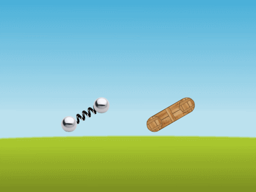
As described in Section 2, use the keyboard to select various bodies and watch how they respond to random impulses. Note that the bodies made from springs will deform when they hit the edges of the window but the bodies made from wood will not (see Fig. 2 for an example). If you apply an impulse to the ragdoll robot and let it lie on the bottom of the window for a second or two as shown in Fig. 3, then it will attempt to self-right and move to the center of the window by applying impulses to parts of its body.

Fig. 2: Deformation of bodies with springs.

Fig. 3: The robot at rest.

5. Code Breakdown

The most important parts of this code are Verlet integration (Section 5.1), Jacobi-Gauss-Seidel relaxation (Section 5.2), and bodies made up of points, sticks, and springs (Section 5.3).

5.1 Verlet Integration

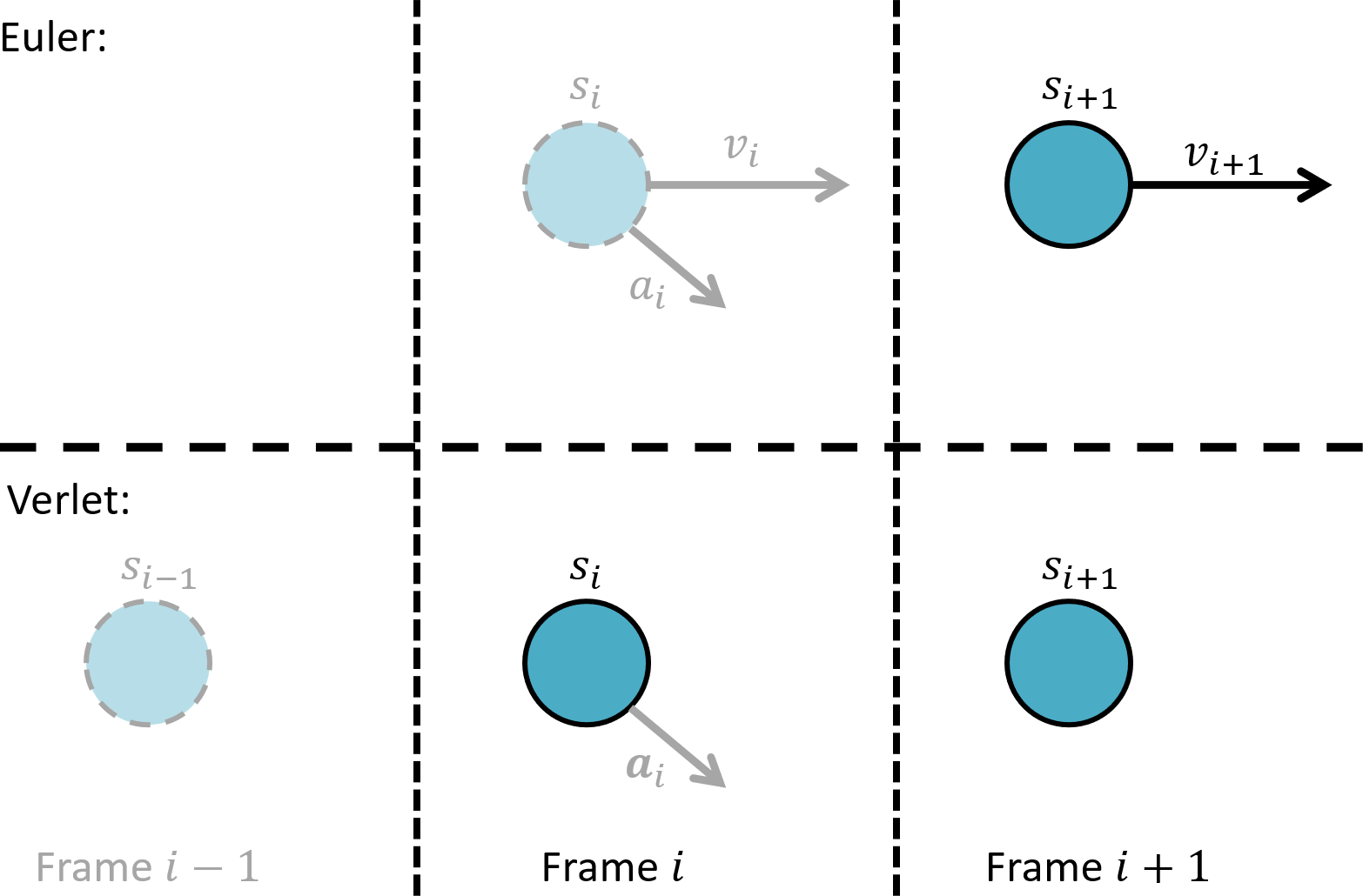
Loup Verlet developed the concept that is now called Verlet integration for use in particle physics simulation. There are mathematical reasons for using Verlet integration instead of Euler integration when simulating systems of particles. One useful feature of Verlet integration is that it is easy to incorporate constraints, which means that Verlet integration makes it easier to code soft-body animation.

Let \(\vec{s}_i\) be the position of a point at the end of frame \(i\), \(\vec{v}_i\) its velocity, and \(\vec{a}_i\) its acceleration, and \(t_i\) be the fixed frame duration. Suppose we know \(\vec{a}_i\), \(\vec{s}_i\), \(\vec{s}_{i-1}\) and want to compute \(\vec{s}_{i+1}\). Let \(\delta_i = \vec{s}_i - \vec{s}_{i-1}\), the distance moved in frame \(i\). The distance to be moved in frame \(i+1\) is

\[\delta_{i+1} = \vec{v}_i t_i + \vec{a}_i t_i^2/2.\]

Now, \(\delta_i\) is a good approximation to \(\vec{v}_i t_i\), and therefore

\[ \delta_{i+1} = \delta_i + \vec{a}_i t_i^2/2. \]

Since \(\vec{s}_{1+1} = \vec{s}_i + \delta_{i+1}\), substituting for \(\delta_{i+1}\),

\[ \vec{s}_{i+1} = \vec{s}_i +\delta_i + \vec{a}_i t_i^2/2. \]

Substituting for \(\delta_i\), we get

\[ \vec{s}_{i+1} = \vec{s}_i + (\vec{s}_i - \vec{s}_{i-1}) + \vec{a}_i t_i^2/2, \]

that is,

\[ \vec{s}_{i+1} = 2\vec{s}_i - \vec{s}_{i-1} + \vec{a}_i t_i^2/2. \tag{1} \]

This shows us how to compute \(\vec{s}_{i+1}\) given \(\vec{a}_i\), \(\vec{s}_i\), and \(\vec{s}_{i-1}\). Notice that there is no need to store velocity. We can even fake a kind of friction in the \(Z\) direction using

\[ \vec{s}_{i+1} = 1.99\vec{s}_i - 0.99\vec{s}_{i-1} + \vec{a}_i t_i^2/2. \]

Recall that in the Shapes Library, the class CDynamicCircle has a private member variable m_vVec that stores its velocity vector \(\vec{v}_i\) in frame \(i+1\). This is used in its move function to compute its new position using the equation

\[ \vec{s}_{i+1} = \vec{s}_i + t_i\vec{v}_i. \tag{2} \]

This method is commonly referred to as Euler integration. Contrast this with Equation (1) above for Verlet integration. Fig 4. summarizes the differences between Verlet and Euler integration.

Fig. 4: Verlet integration.

We can optimize Equation (1) by assuming that \(t_i\) is a constant (in fact we can make it equal to \(1\)), ignoring the division by 2 and increasing \(\vec{a}_i\) to compensate, ending up with

\[ \vec{s}_{i+1} = 2\vec{s}_i - \vec{s}_{i-1} + \vec{a}_i, \]

or, if there is no acceleration,

\[ \vec{s}_{i+1} = 2\vec{s}_i - \vec{s}_{i-1}. \tag{3} \]

We implement this in class CPoint which has two private member variables CPoint::m_vPos and CPoint::m_vOldPos. CPoint::move computes the new value of CPoint::m_vPos as follows:

const Vector2 vTemp = m_vPos;
m_vPos += m_vPos - m_vOldPos; 
m_vOldPos = vTemp;

Notice that the second line of the above code implements Equation (3). It uses only four floating point additions, whereas Equation (2) requires four floating point additions and two floating point multiplications. Acceleration due to gravity is then faked by:

m_vPos.y -= 0.2f;

5.2 Jacobi-Gauss-Seidel Relaxation

We mentioned in the previous section that Verlet integration makes it easy to enforce constraints on points. We can model a stick by applying Verlet integration to two points at its ends. The constraint is that the distance between the points must remain constant. We can move the stick by moving each point independently, then trying to correct their positions to satisfy the distance constraint (before rendering) if they are the wrong distance apart.

Fig. 5: A stick represented by two points.

Fig. 6: The vector from one point to the other.

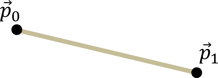
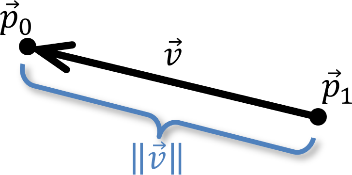
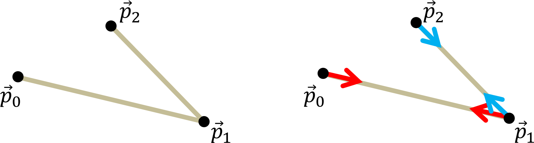
Suppose we have a stick of length \(d\) whose end points are at positions \(\vec{p}_0\) and \(\vec{p}_1\) after they have been moved independently as shown in Fig. 5. Let \(\vec{v} = \vec{p}_0 - \vec{p}_1\) be the vector from \(\vec{p}_1\) to \(\vec{p}_0\) as shown in Fig. 6 and let us suppose that \(\Vert \vec{v} \Vert \not= d\). We will displace the end points along the stick by an equal amount so that the distance between them is \(d\).

Fig. 7: Correcting the length of the stick.

Define

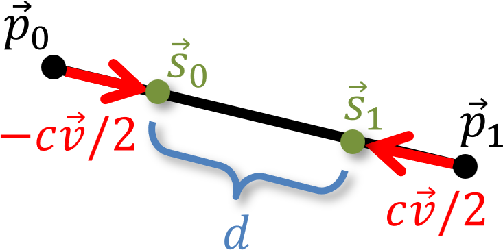
\[ c = 1 - d/\Vert\vec{v}\Vert \tag{4} \]

. Let the new end points of the stick be \(\vec{s}_0 = \vec{p}_0 - c\vec{v}/2\) and \(\vec{s}_1 = \vec{p}_1 + c\vec{v}/2\) as shown in Fig. 6. The length of this stick is then \(\Vert\vec{s}_0 - \vec{s}_1\Vert = \Vert\vec{v}\Vert -(1-d/\Vert\vec{v}\Vert)\Vert\vec{v}\Vert = d\). This process is called relaxation.

Fig. 8: Two joined sticks with three points.

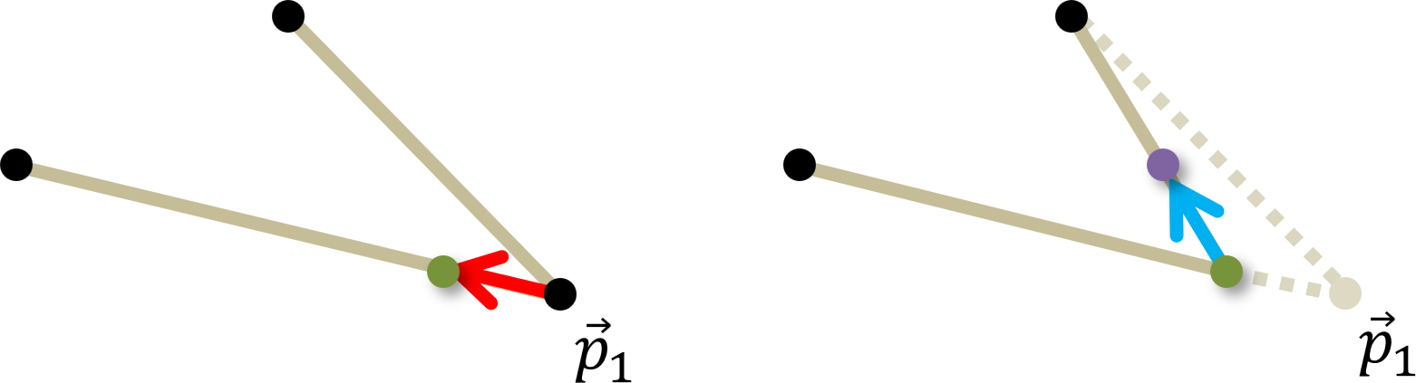
Now suppose that we have two sticks with one end point in common such that they can freely rotate about this point. Suppose one stick has end points \(p_0\) and \(p_1\), and the other stick has end points \(p_1\) and \(p_2\) as shown in Fig. 8, left. Further suppose that both sticks have the wrong length and need to be corrected as shown in Fig. 8, right. We could try relaxing one stick and then the other, but the result will be wrong as shown in Fig. 9. The shared point \(\vec{p}_1\) will be first moved to the green point in Fig. 9, left, then to the purple point in Fig. 9, right. As we see in in Fig. 9 right, the purple point is not on the stick with end points \(p_1\) and \(p_2\).

Fig. 9: Sequential relaxation gives the wrong result.

However, if we repeatedly relax first one stick then the other, the end points will eventually get very close to where they need to be. This was independently discovered by the mathematicians Jacobi, Gauss, and Seidel, thus the name Jacobi-Gauss-Seidel relaxation_. Rather than checking for closeness (which would be computationally very expensive), we will just do a small fixed number of iterations and hope for the best.

Furthermore, we can implement springs as well as sticks by replacing Equation (4) with

\[ c = r(1 - d/\Vert\vec{v}\Vert) \tag{5} \]

where \(0 < r \leq 1\) is called the restitution, which is a measure of the stiffness of the spring, where a stick has restitution 1.

In our code each point will be implemented as an instance of CPoint. CPoint::move moves the point using Verlet integration (see Section 5.1) Each spring will be implemented as an instance of CSpring. CSpring::Relax performs one iteration of Jacobi-Gauss-Seidel relaxation using Equation (5). Sticks will be instances of CSpring with private member variable CSpring::m_fRestitution = 1.

5.3 Bodies

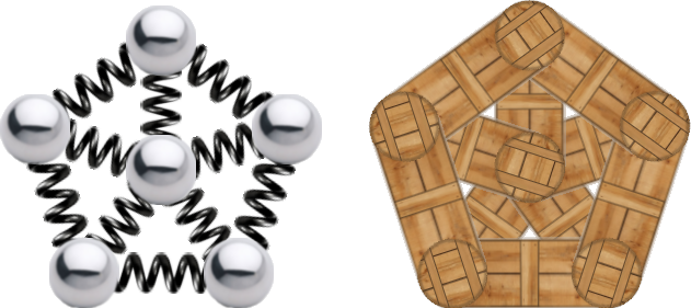
A body is a collection of points and springs connecting those points. It will be represented as an instance of CBody, which has member variables made up of pointers to instances of CSpring and CPoint. There are three kinds of body, each of which is derived from CBody. CChain is a chain of connected points, as in Fig. 10. Note that there are two instances of CBody drawn there, one made up of sticks and the other springs. Successive levels show chains of 2, 3, and 4 points. CChain consists of just a constructor that puts the points in the right position and connects them with sticks or springs as required.

Fig. 10: Three-point chains made of sticks (left) and springs (right).

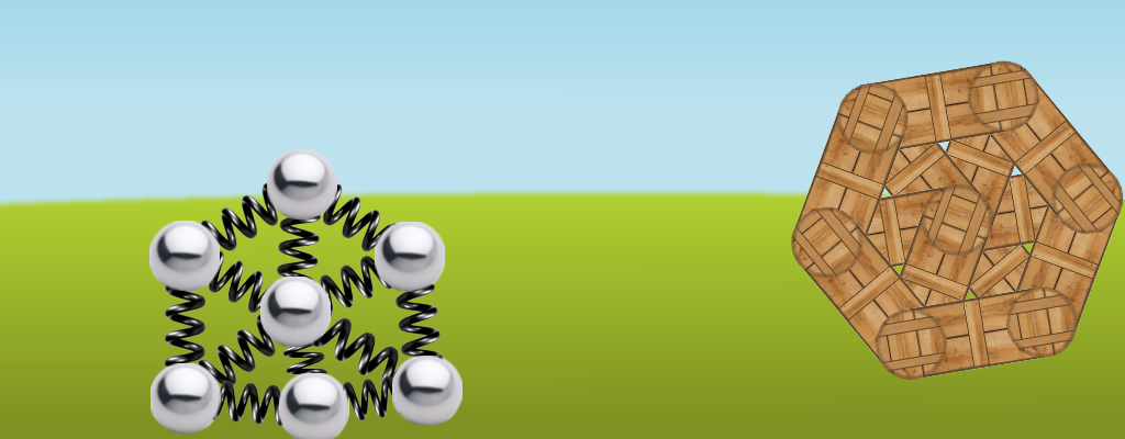
CWheel is a circle of points connected to a central point which acts as a hub. Successive levels show wheels that are square, pentagonal, and hexagonal. Fig. 11 shows a pentagonal wheel. CWheel consists of just a constructor that puts the points in the right position and connects them with sticks or springs as required.

Fig. 11: Pentagonal wheel made of sticks (left) and springs (right).

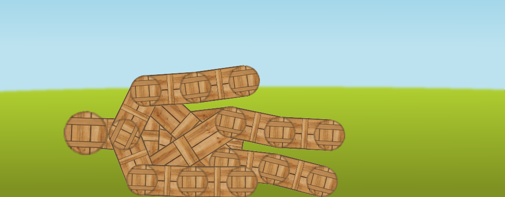
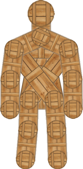
Finally, Woody the ragdoll robot (see Fig. 12) is an instance of CRagdoll made up of both sticks and springs. In addition to the constructor, CRagdoll has various functions that implement the rule-based AI that makes it jump back onto its feet after it has fallen (see Fig. 3).

Fig. 12: Woody the ragdoll robot.

6. Problems

For the following problems you can either work directly in the folder 5. Ball and Spring Toy in your copy of the sage-physics repository, or (recommended) make a copy of the folder 5. Ball and Spring Toy in some place convenient (for example, the Desktop or your Documents folder) and work there.

Problem 5.1

Modify the code so that it works as follows. Hitting the down arrow (VK_DOWN) must scale the objects by 4/5 each time it is hit, down to a minimum of 16/25. Hitting the up arrow (VK_UP) scale the objects by 5/4 each time it is hit, up to a maximum of 1. The object must relaunch each time you scale up or down. For example, Fig. 13 shows the first body in their scaled initial positions at small (scale factor \(0.75^2\)), medium (scale factor \(0.75\)), and large (scale factor \(1\)) scale.

Fig. 13: Scaled object in the initial position for small, medium, and large.

Hint:

Begin by adding a new static member variable m_fScale to CCommon, initialized to 1.0f. Add the following code to CGame::KeyboardHandler:

const float fScaleFactor = 0.8f;
const float fScaleFactorSq = sqr(fScaleFactor);

if(m_pKeyboard->TriggerDown(VK_UP) && m_fScale < 1.0f){ 
    m_fScale = min(1.0f, m_fScale/fScaleFactor);
    BeginGame();
} //if

if(m_pKeyboard->TriggerDown(VK_DOWN) && m_fScale > fScaleFactorSq){
    m_fScale = max(fScaleFactorSq, m_fScale*fScaleFactor);
    BeginGame(); 
} //if

The main things that must scale by CCommon::m_fScale are the initial position (as shown in Fig. 13), gravity, collision detection and response, sprite scale (as shown in Fig. 13), impulse magnitude, and ragdoll AI.

7. What Next?

Next, take a look at the Box2D Render Library.